Research
Pendulum Static
Open Loop
Optimal Static-> Static
Optimal Control: Static->Static
Periodically Driven (but NON Chaotic regime)
Double Pendulum Optimal Control
Chaos Control
Pendulum
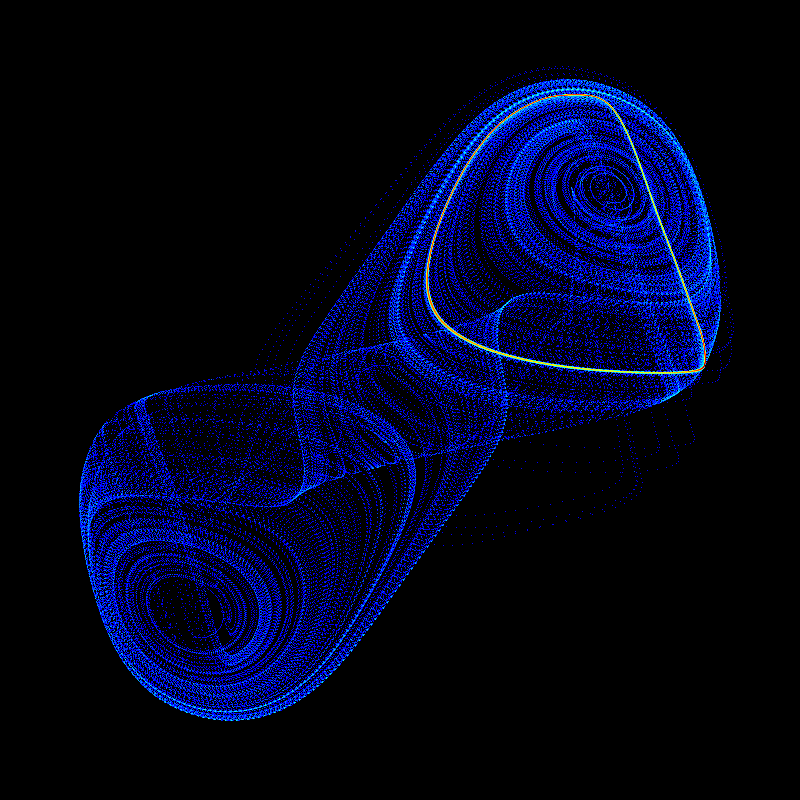
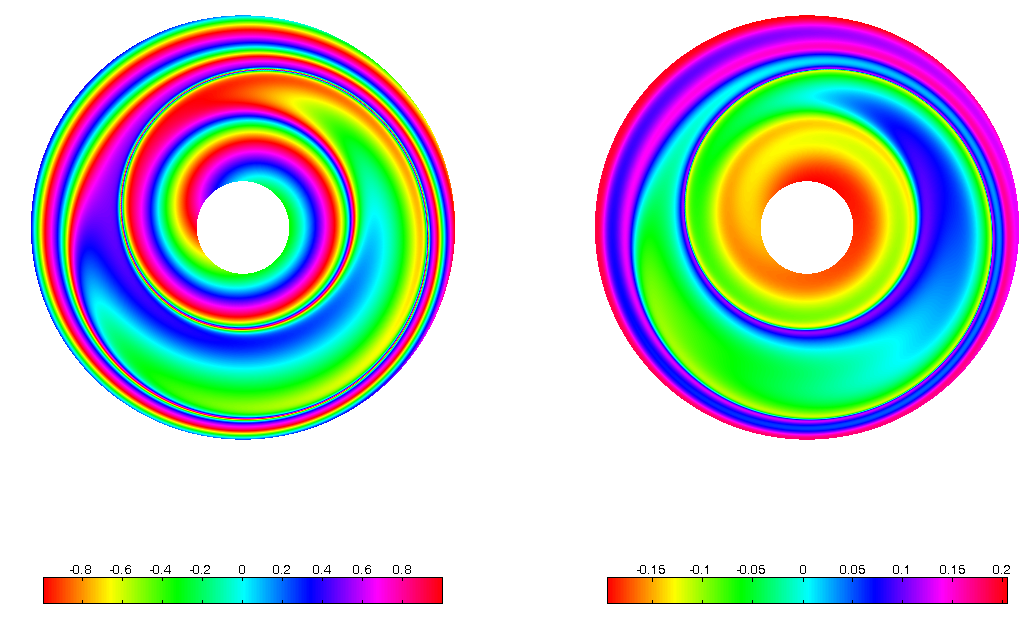
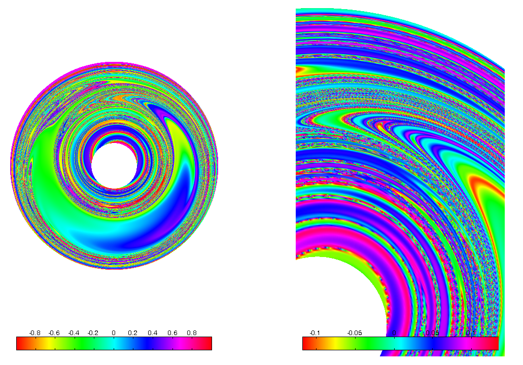
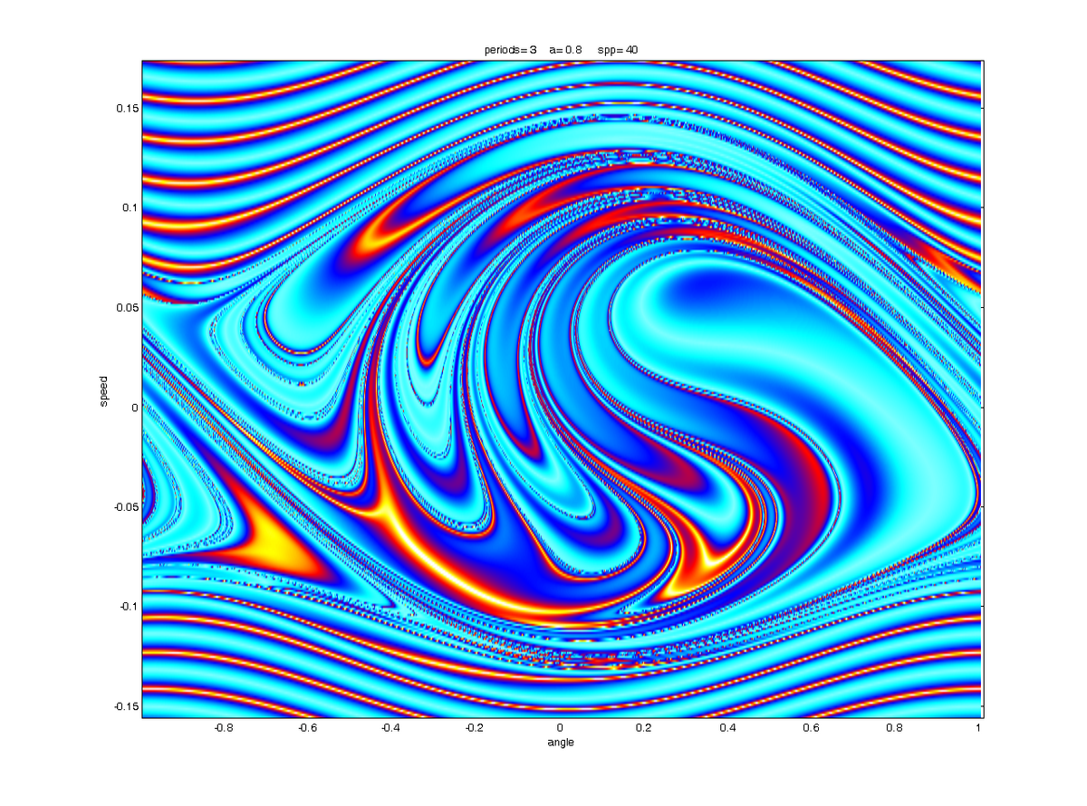
Strange Attractor of Driven Pendulum
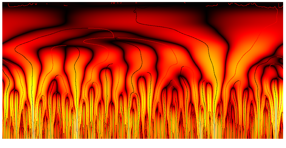
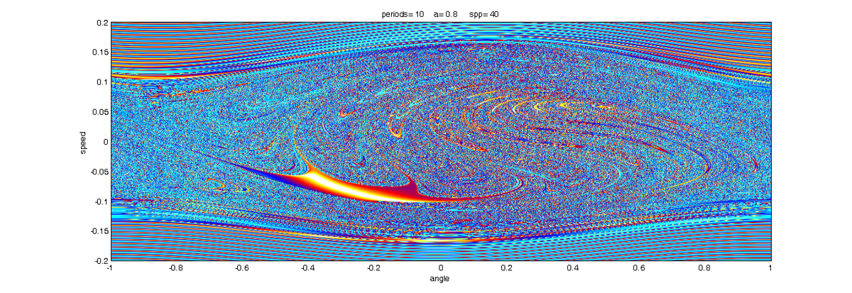
Route to Chaos
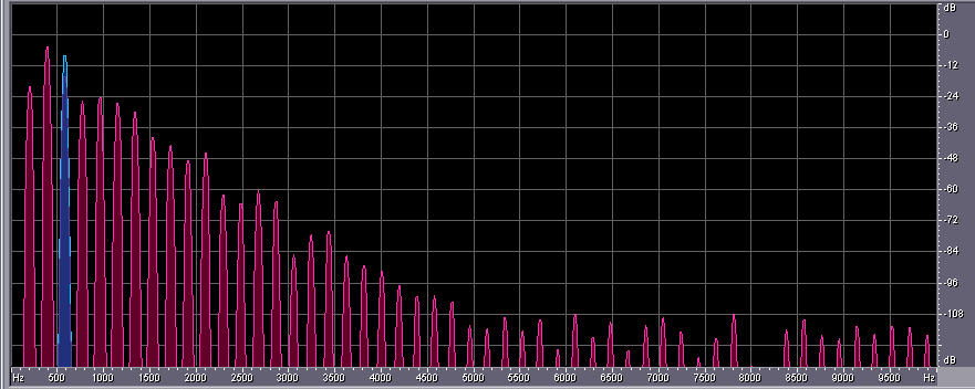
Depending on parameters like frequency and amplitude of the driving sled, the pendulum can show up different behaviour. Typical "pre-stages" of chaos are period-doubling, period tripling etc. orbits, which are shown below. The sound you can hear and which is displayed in the spectra below corresponds to the angular speed signal of the pendulum, with time scaled by a factor 1000.
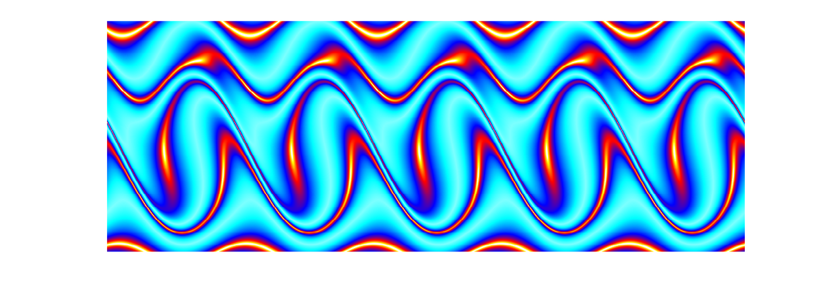
Sine of driving position, corresponding to blue spectral lines below
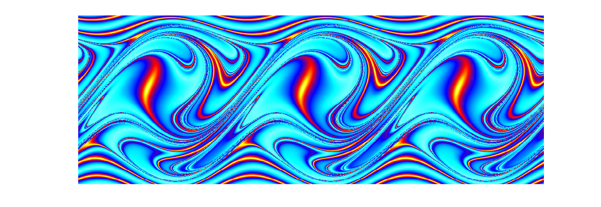
Speed signal in period doubling case. An octave BELOW the driving signal above!
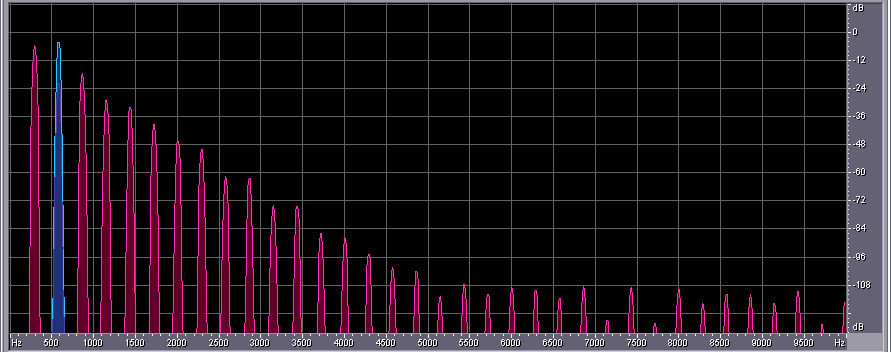
Period Doubling Spectrum
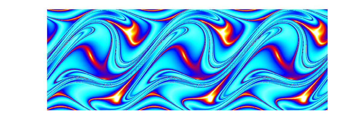
Speed signal in period tripling case. A duodezim BELOW the driving signal above!
Period Tripling Spectrum
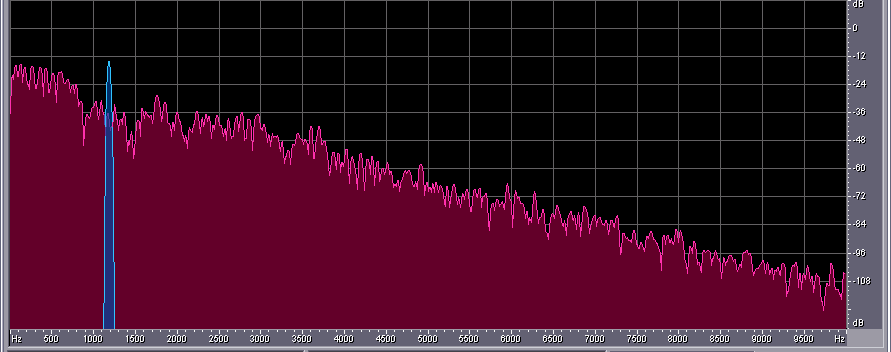
Chaotic Pendulum. Speed Signal shows a 1/f- Noise behaviour
Spectrum of speed signal in chaotic case (driving frequency (blue) higher than in examples above)
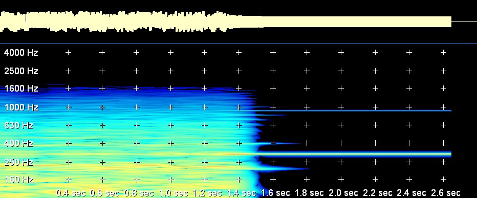
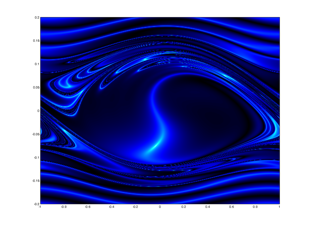
Transient Chaos
For some parameter sets the strange "attractor" is no attractor anymore (yet an invariant set of the flow). After some (unpredictable) time the system switches back to a stable periodic orbit.
Transient (i.e. instable) Chaos
Spectrogram for transient chaos: System switches to stable periodic orbit
Strange Attractor of Driven Pendulum
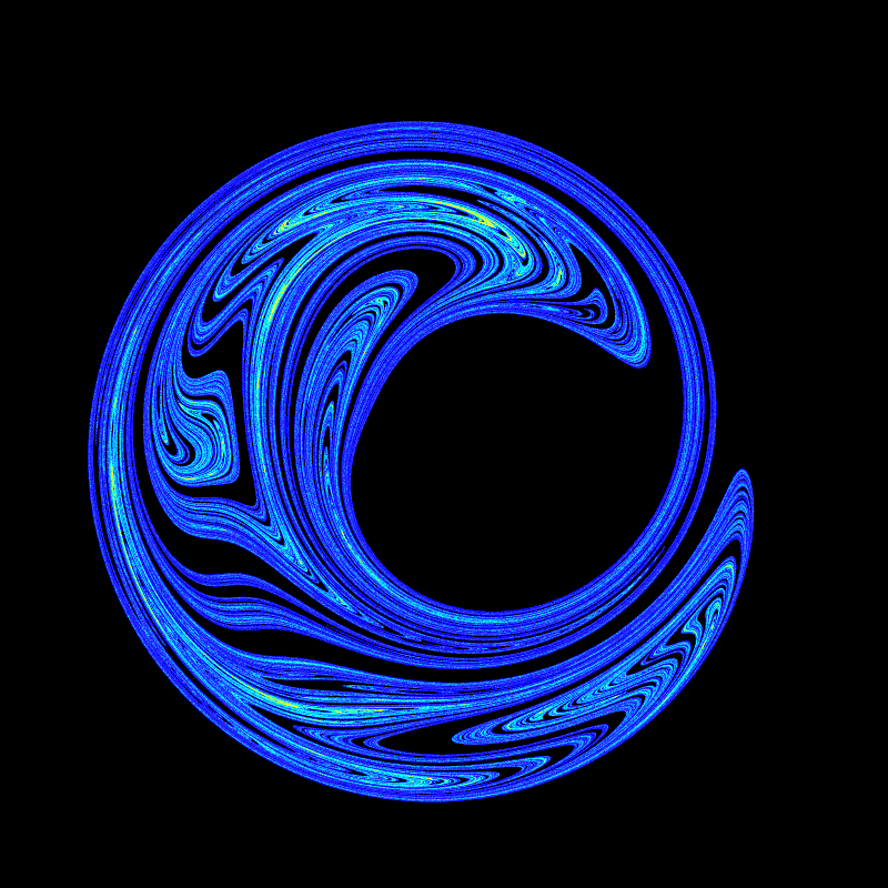
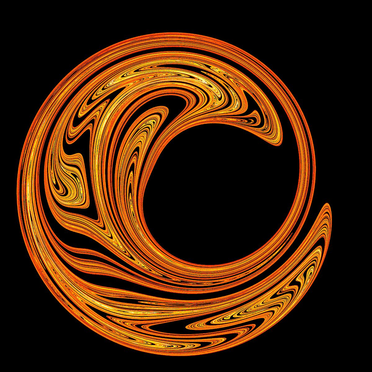
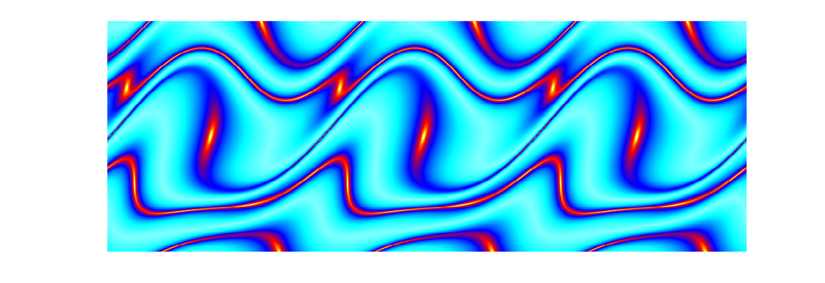
Chaotic Pendulum Art Gallery
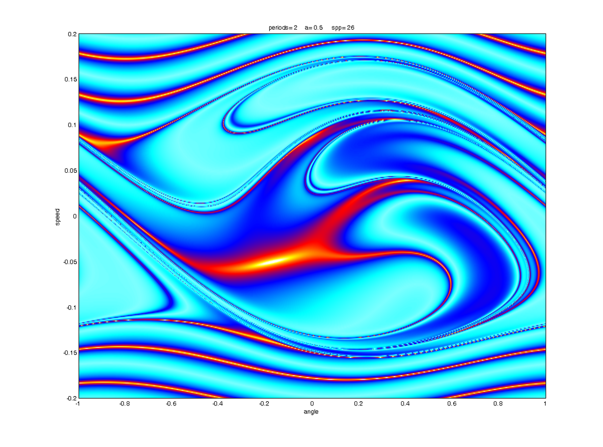
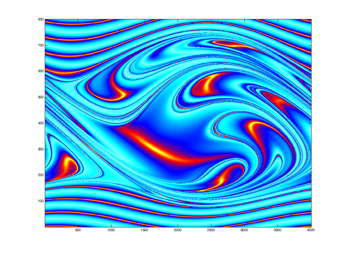
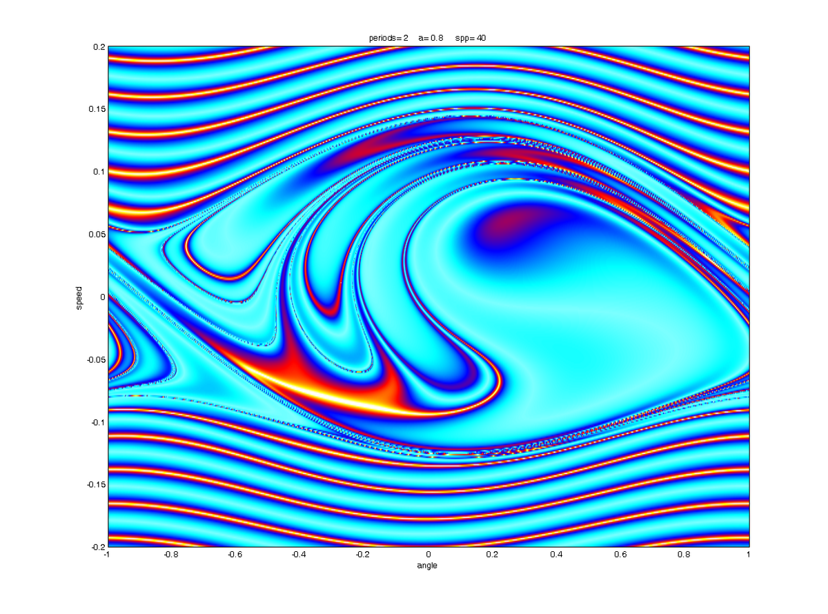
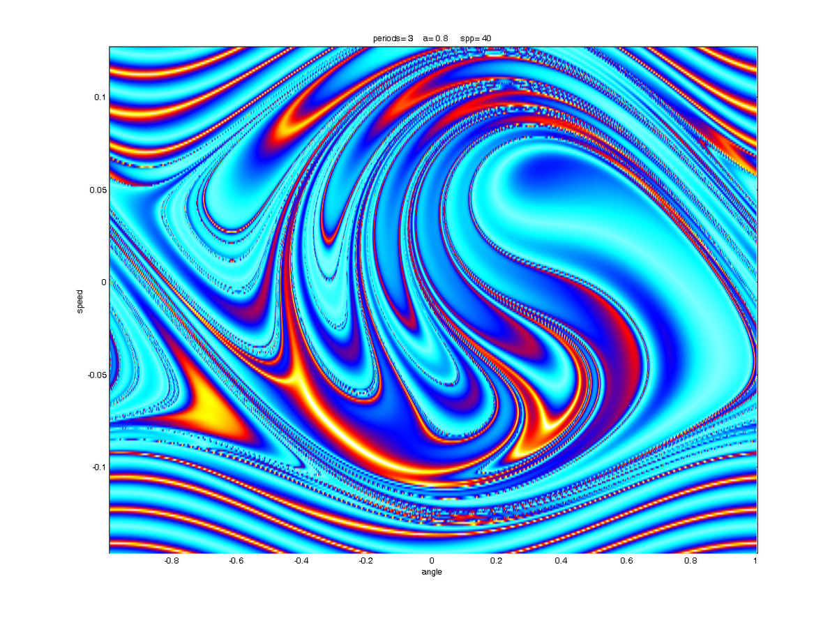

Chaos Control: Various UPOs
Chaos Control: Left-Right Transient example
Uncontrolled Chaos
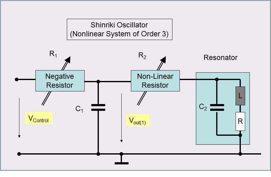
Modified Shinriki
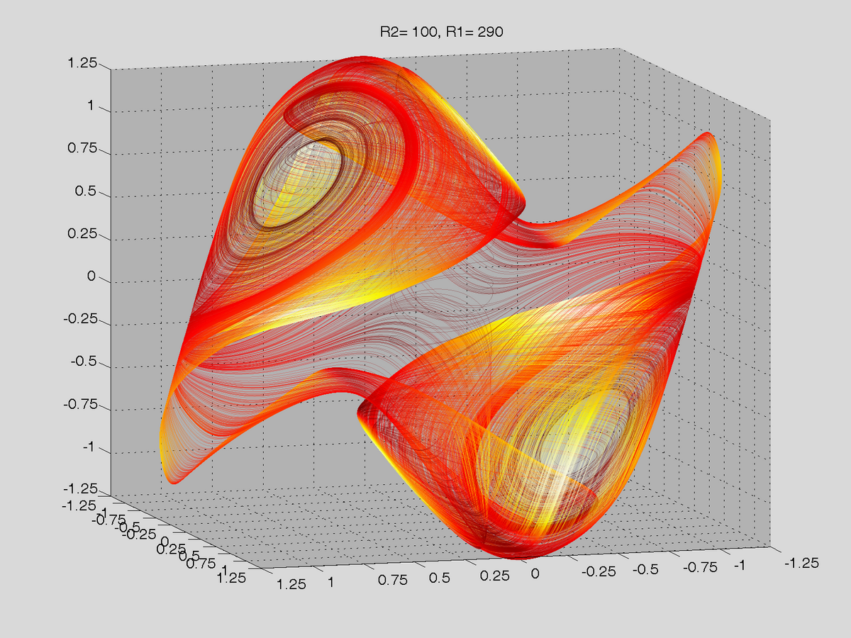
Strange Attractor of Modified Shinriki Oscillator
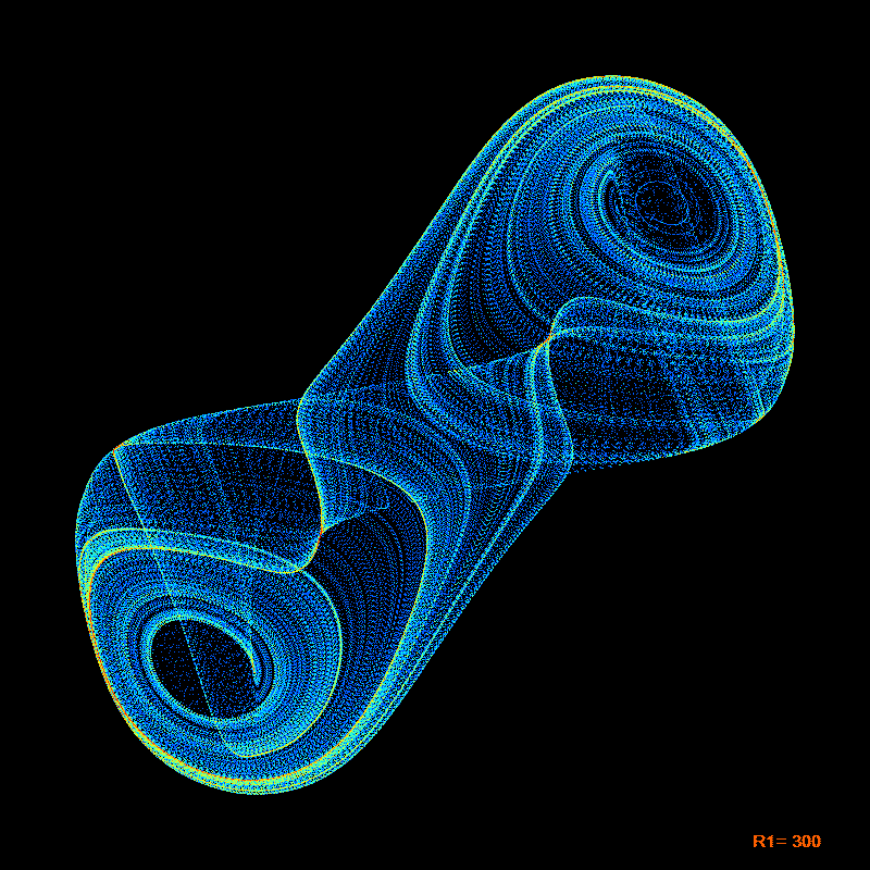
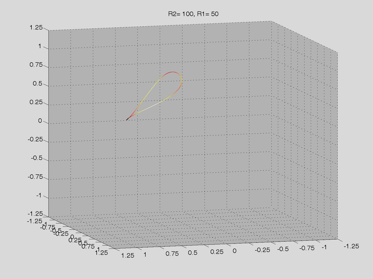
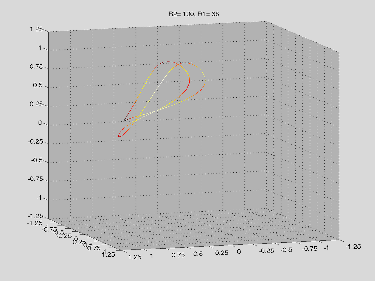
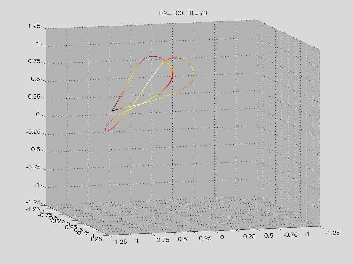
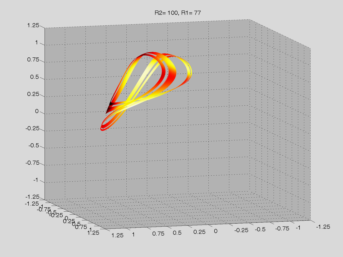
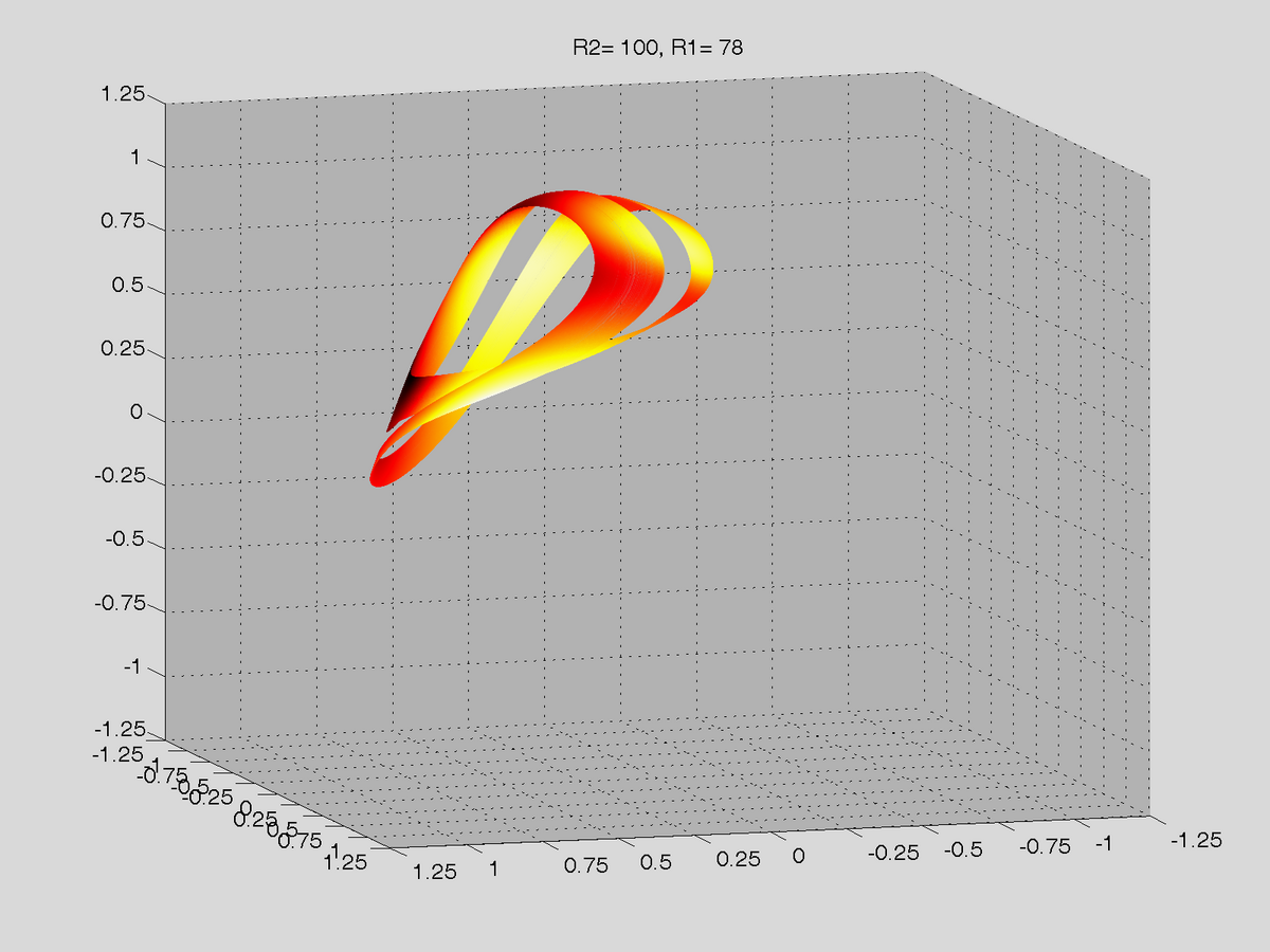
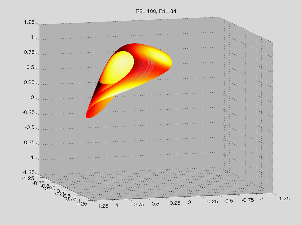
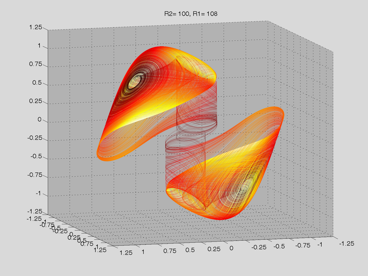
Measured strange attractor R1=300
Click image to see attractor for different values of R1
Experimental setup
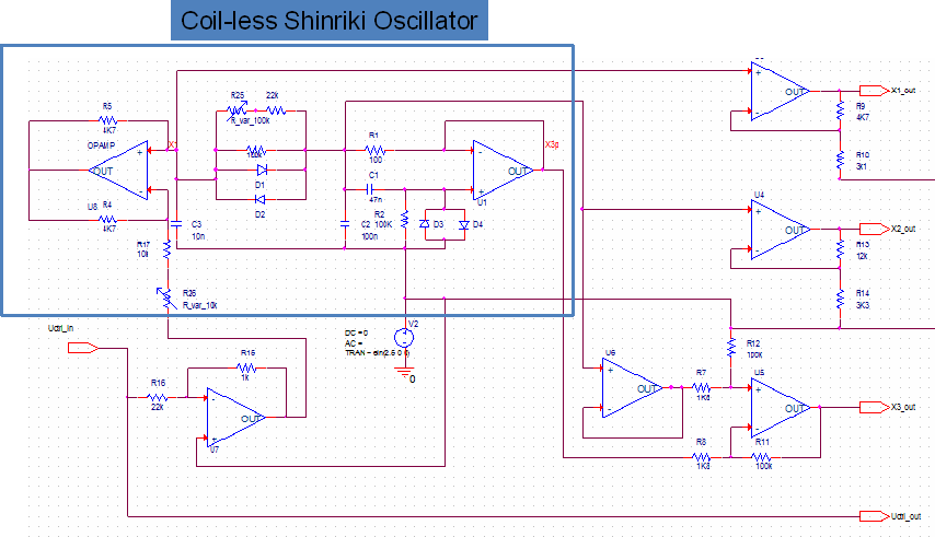
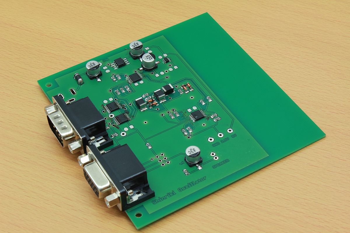
Coil-less Shinriki-type Oscillator
During a student's project a coil-less chaotic oscillator operating at a single 5V supply has been designed and realized. The non-linearity consist of two anti-parallel diodes, thus the I-V behaviour is well described by a hyperbolic sine function. The rest of the circuit is linear, which allows for a simple mathematical description and makes numerical simulations is easy. Parameters of the oscillator are the resistors R1 and R2, which are implemented as digitally programable integrated circuits. Thus, fully automated measurements of attractors using an USB DAC device are possible. Furthermore, chaos-control experiments in real-time can be performed, using a programmable (fix-point) DSP device in conjunction with ADCs and DACs.
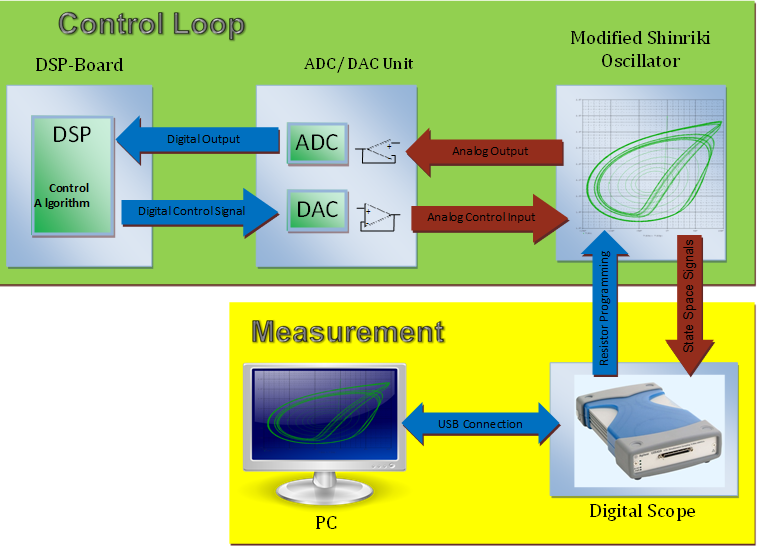
Block Diagram
Principle block diagramm of controlled Shinriki oscillator. Note that the inductivity is replaced by an OP-amp circuit in our modification.
Schematic of modified Shinriki Oscillator including I/O buffering
Block Diagram
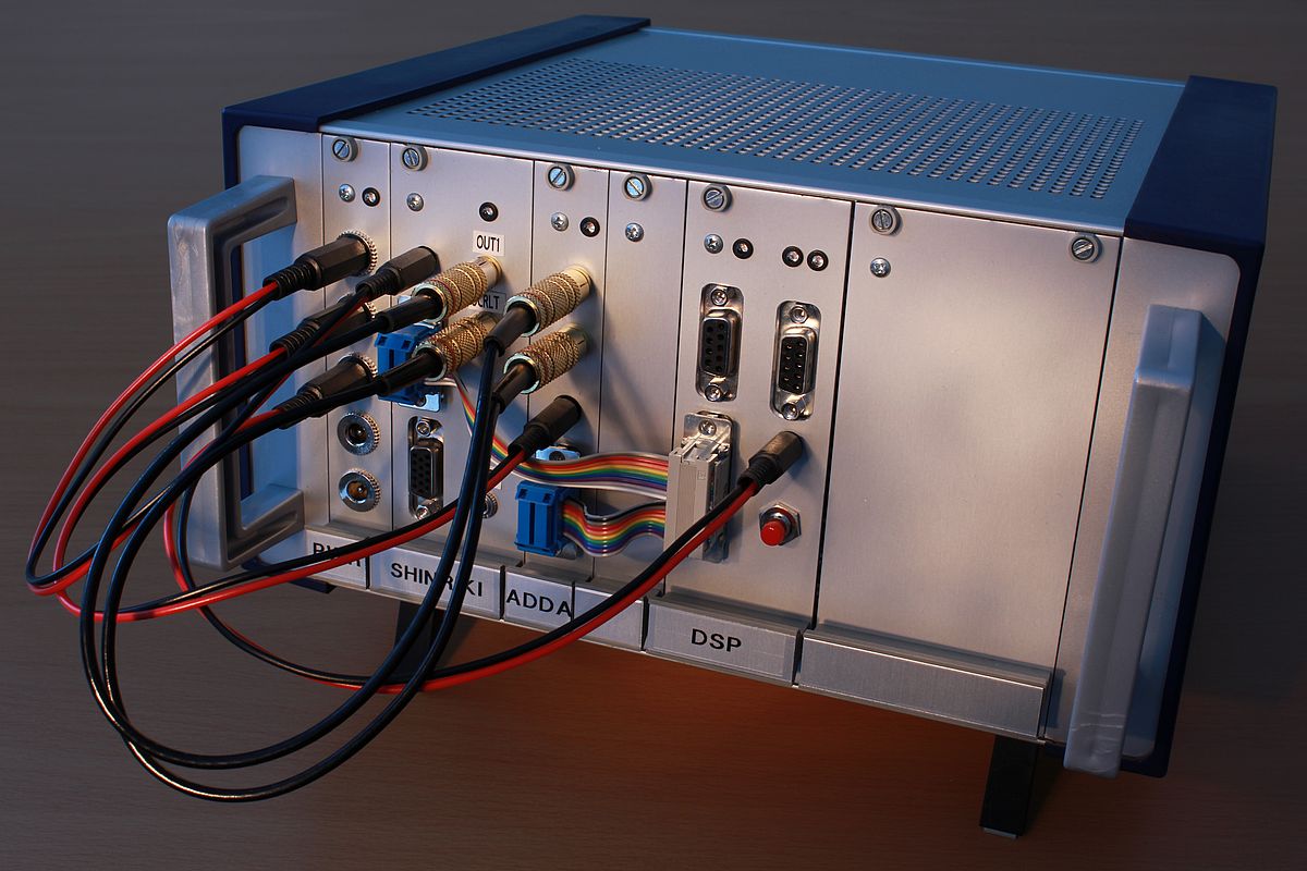
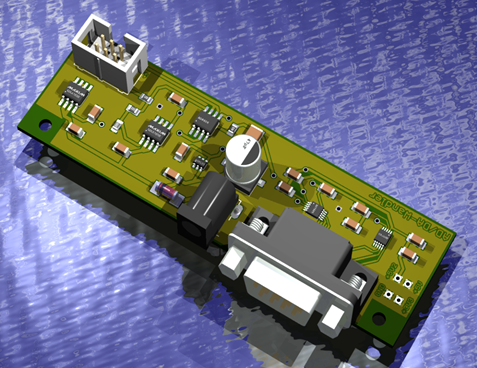
Hardware Realization
Chaos Control for Modified Shinriki Oscillator
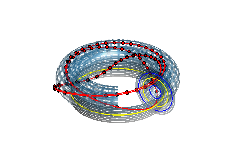
UPOs embedded in strange Attractor
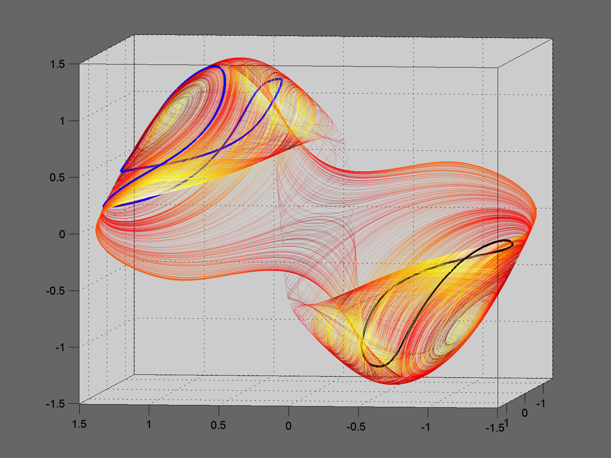
The strange attractor of the Shinriki oscillator contains (infinitely many) unstable periodic orbits (UPOs). One of the goals of chaos control is to stabilize them. In the figure the attractor is shown in its full 3 dimensional phase space together with two (stabilized) UPOs: Period 2 (blue) and period 1 (black). Data are from actual measurements, not from simulation!
Simple TDFC scheme
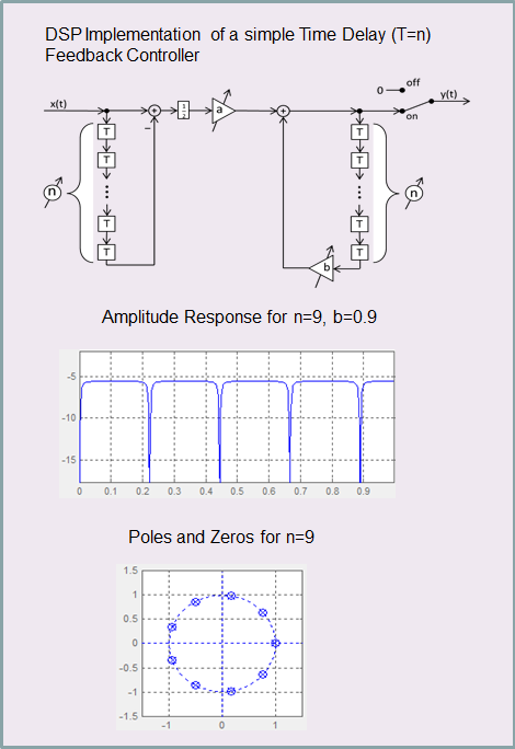
One of the simplest ways to control a chaotic system is Time Delay Feedback Control (TDFC). From point of view of signal processing this corresponds to a periodic notch-filter, as shown to the left. The advantage of this type of control is - besides its simplicity of implementation- that the system dynamics of the chaotic oscillator needs not to be known in detail. Only the period duration n needs to be known exactly, in order to obtain a truly vanishing control signal. To this end, the sampling frequency must be choosen rather high, allowing for fine tuning of the delay time. A more sophisticated controller, including also automatic period locking, is discussed below.
TDFC Measurement Results
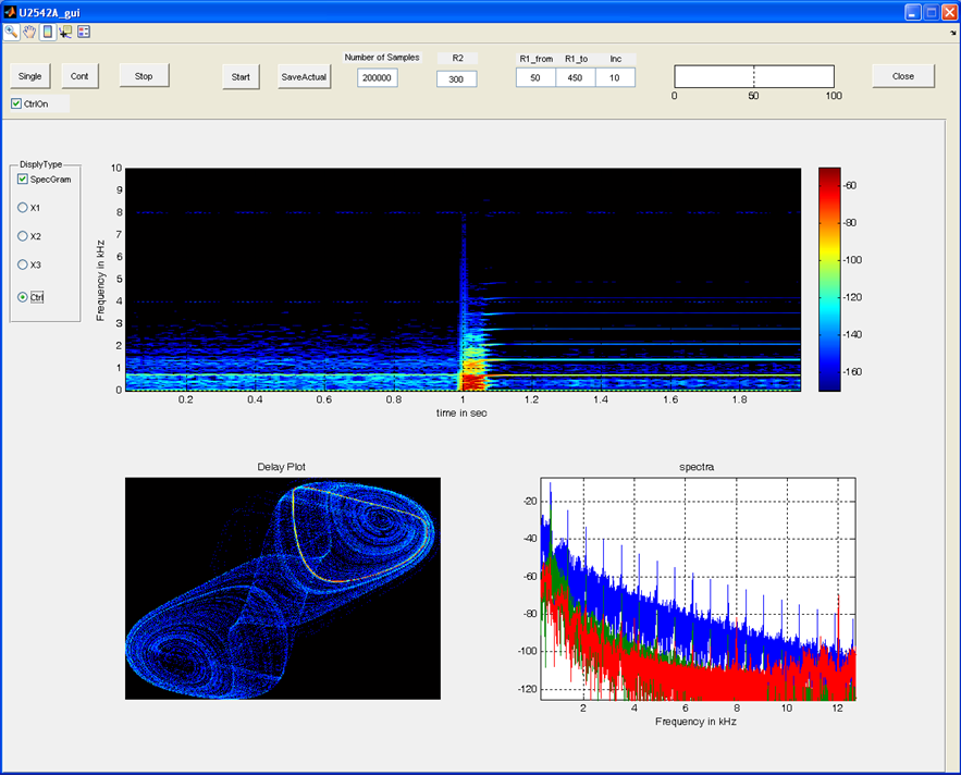
GUI for TDFC measurement. In the first picture, a spectrogram of the Shinriki-State-Signal x1 is displayed. Clearly, the orbit becomes perfectly periodic. The phase image contains both, the trajectories from the chaotic attractor (0...1sec) and the embedded period one UPO (from data 1..2sec). Lower right are Fourier spectra, clearly showing discrete lines as proof for periodicity.
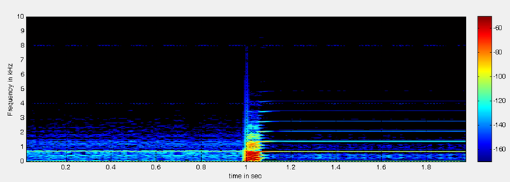
The corresponding spectrogram of the control signal shows some "strong action" shortly after activating control (t = 1sec), followed by a quick decay of energy. Note that the total power after having stabilized the periodic orbit is well below -80dB (!), wheras the state signal x1 has power of around -10dB.
Similar scenario as above, showing a "zoom" of the control signal in time domain. At sample time 500 the controller was activated, most of the "work" is done after a few periods (of the UPO to be stabilized).
Signal Processing Implementation of TDFC
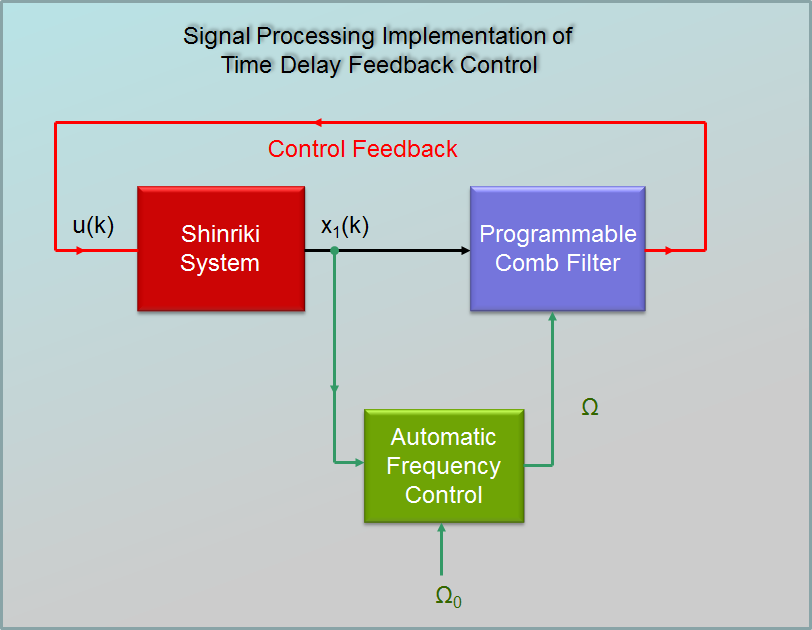
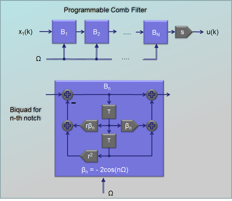
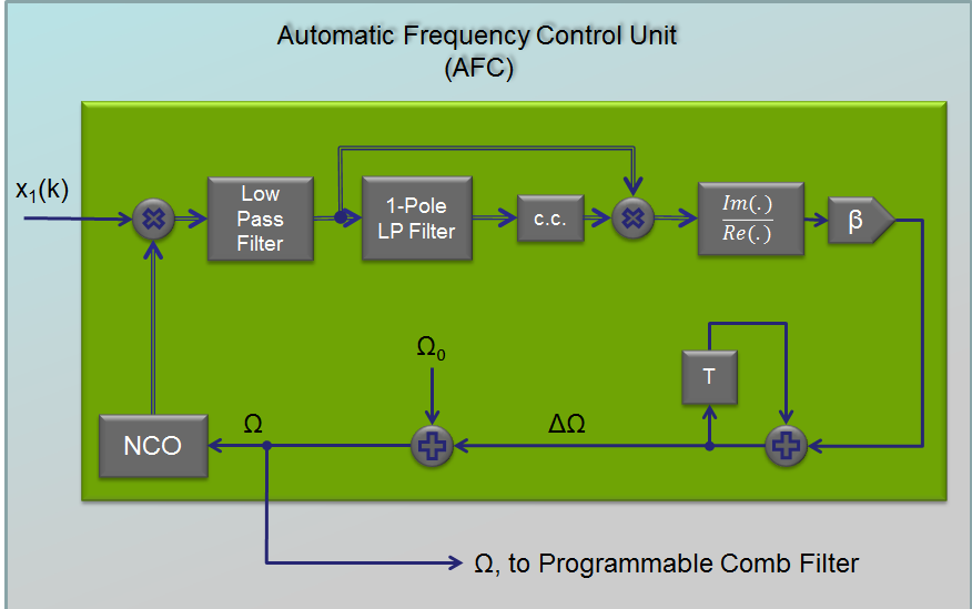
The simple time delay implementation discussed above has the disadvantage that the sampling rate must be choosen rather high, in order to have a low enough granularity for the delay time. From point of view of signal processing, a sampling frequency which catches, say, the 8th harmonic of the periodic signal, is completely sufficient, since the spectra decay relatively fast with frequency.
The controller can thus be realized as a programmable comb filter with notches at Ω, 2Ω, 3Ω,... . Each notch is implemented as a biquad section comprising a zero-pole pair. The fundamental frequency Ω is then controlled by an AFC (automatic frequency control) algorithm, which operates in the baseband (double-line arrows are complex signals). With this circuit we can easily stabilize all kinds of UPOs, also with higher periods and also in a wider range of parameters R1 and R2. The AFC locks in a relatively wide frequency-range around the nominal point Ω0.
Route to Chaos
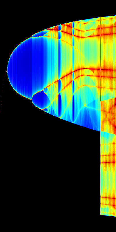
The Shinriki Oscillator shows up very different behaviour, depending on parameters. Starting a stable fix-point we watch a period doubling cascade, arriving at a strange attractor. Intermediate stable period 3 and period 5 orbits (and more) show up, finally arriving in a double-D strange attractor. As seen in the fig-tree representation, we find stable orbits also inside "chaotic parameter ranges" (e.g.of R2).
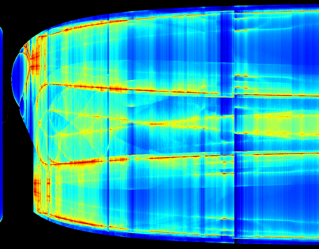
Fig Tree
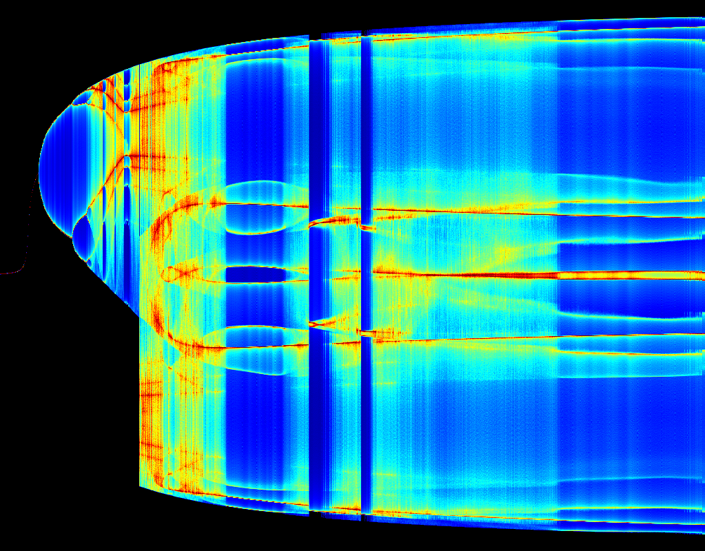
Colors represent probability distribution of state variable x1, as function of R1 (R2=200). (Image created from measured data!)
Animation: R1 varies with time (R2=200)
Measured strange attractor R1=300
Click image to see attractor for different values of R1
Full Phase Space Orbits for various R1


Gallery: Attractors and Fig Trees